Tree Problem

Brenda King

Tree Problem

The problem:

Using data from the lumber industry which gives the approximate number of board feet of lumber per tree in a forest of a given age, find a function that will fit the data. Predict the harvest for ages other than those given.

Age of Tree	100s of Board Feet
20	1
40	6
60
80	33
100	56
120	88
140
160	182
180
200	320

Introduction

In many real-world problems there exist patterns or relationships between sets of numerical data. The relationship among the data can be influenced by many variables. In the case of trees, the variables may include age, soil condition, weather, insects, and human intervention. In this investigation, the relationship between Age of Trees and number of 100s of board feet will be modeled.

How can a model be fit to data? How can the “best” model be selected? Can the model be used to predict values other than those given? Are there limits on the use of the model?

Examining Relationships

An effective way to see a relationship in data is to display the information in a scatter plot. A scatter plot shows how two variables relate to each other by looking for patterns in the data. Strong relationships show data following a specific pattern or trend and weak relationships show data widely dispersed or with no pattern at all. The scatter plot for the tree data is shown in diagram 1.

Diagram 1

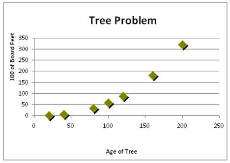
Scatterplots show the form and strength of the relationship between sets of data. For the tree problem, the data moves in a positive direction from the lower left corner to upper right corner of the graph. The form of the relationship is slightly curved. The strength of a relationship is determined by how closely the points follow the curve. The tree scatterplot seems to indicate a strong relationship. A model can be constructed to represent this data.

When the points in a scatter plot are represented by a line of best fit, the line can be used to predict values other than the ones given. Linear relationships are quite common and simple to use. Since the scatterplot displayed for the tree data appears to be curved, the function model will probably not be linear. Many statistical measurements, such as correlation r, are based on the strength of a straight-line relationship. In order to use these measures to determine the “best” model, a transformation will be necessary to achieve linearity.

Curve fitting

The process of fitting a set of data with a model can be done in many ways.

For example, given three noncollinear points, a quadratic model can be fit to the data. To find a, b, and c in f(x)=ax²+bx+c, write and solve a system of three linear equations using the three unknowns.

Three data points were selected from the tree problem and setup in equations as shown below.

Point	Substitution	Equation
(20,1)	a(20)²+b(20)+c = 1	400a+20b+c=1
(80,33)	a(80)²+b(80)+c = 33	6400a+80b+c=33
(160,182)	a(160)²+b(160)+c = 182	25600a+160b+c=182

Using a matrix equation, X=a^-1 b, to solve for a, b, and c, gives the following output:

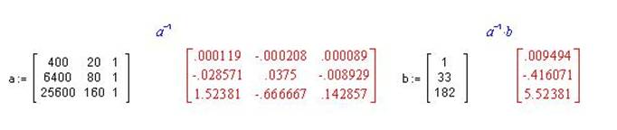
These results produce the quadratic model of f(x) = .009494x². -.416071x + 5.52381.

The graph of the tree data and quadratic model are shown in diagram 2.

Diagram 2

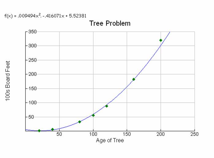
Although this model is not an exact fit, the last point is clearly not on the line, it does look like a nice fit. The equation produced from these three randomly selected points will not produce the only quadratic model for the tree problem. The model is dependant on the points selected for the calculation. If a different set of points are used, the equation would change.

The degree of the polynomial can increase if more points are used. Given four noncollinear points, a quartic model can be fit to the data.

Another way to produce function models is to use graphing calculators or excel spreadsheets. Diagram 3 - 8 are sample models produced in this way.

Diagram 3 Linear

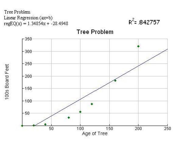
The linear model does not seem to be a good fit, only two points are close to the line.

Diagram 4 Exponential

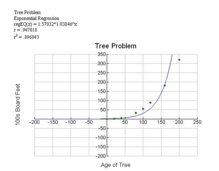
The exponential model does not seem to be a good fit either, however, points are closer to this curve than the linear model.

Diagram 5 Quadratic

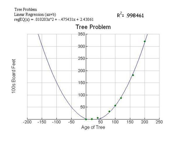
For the models with degree greater than 1 (as shown in diagram 5-8), the domain must be restricted to positive values (tree ages). These diagrams included negative values to better display the shape of the model.

The quadratic model created from the calculator produces a tighter fit, to all the points, than the 3 point model. The calculator has more data to use in the equation.

3 point model: f(x) = .009494x². -.416071x + 5.52381

7 point model: f(x) = .016203x². -.475431x + 2.43061

Diagram 6 Cubic

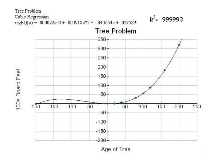
With the increase of each power, the curve appears to be passing through and closer to more and more data points.

Diagram 7 Quartic

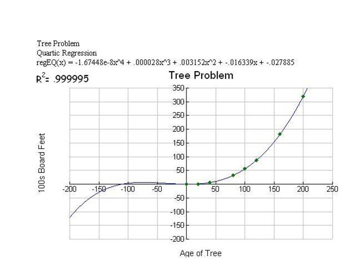
The changes shown in the correlation of determination, R², confirms the improvement of each graph.

Diagram 8 Power

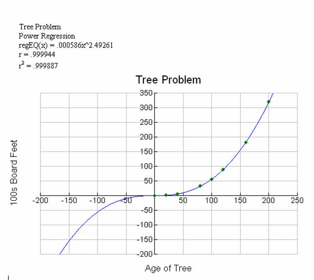
The power model seems to have slipped in the measure of fit as determined by R², but still a very strong relationship is modeled.

Selecting the best model

A correlation coefficient, r. indicates how closely the data points cluster around a linear model. The coefficient of determination, r², is a numerical quantity that tells how well the least-squares line does at predicting values.

When data is nonlinear, a transformation can be done to use correlation measures. One of the transformations that will be described here (to flatten out nonlinear models) is for power equations y=ax^p.

Taking the logarithm of both sides of the power equation gives log y = log a + p log x. The results is a linear relationship between log x and log y. The power p in the power equation becomes the slope of the straight line that links log y to log x. If by taking the log of both variables produces a linear scatterplot, then the results is a reasonable model for the original data.

With the linear model just created, the least-square regression analysis and the measures of good fit, such as correlation, can be used. Diagram 9 shows the linearized Tree data and the graph of the results.

Log (AGE)	Log (Board)
2.995732274	0
3.688879454	1.791759469
4.094344562	2.785608595
4.382026635	3.496507561
4.605170186	4.025351691
4.787491743	4.477336814
4.941642423	4.911544711
5.075173815	5.204006687
5.192956851	5.511128522
5.298317367	5.768320996

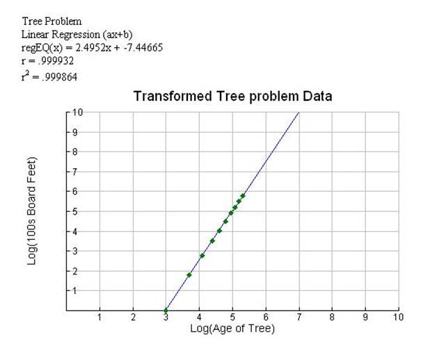
With the correlation of determination, r², set at .999864, we see we have a good fit to the original data. The graphing calculator does provide a correlation of determination with the models shown in diagrams 3-8, but it is also nice to see how a nonlinear curve is “straighten” out for the calculation just done and shown in diagram 9.

Predicting values

Using the model produced in the transformation, f(x)=2.4952x-7.44665, and plugging in log(60), log(140), and log(180) values not given can be predicted. To get the results needed the data is converted back to the original form by using them as an exponent. The table below has been filled in with the missing values.

Age of Tree	100s of Board Feet
20	1
40	6
60	15.95
80	33
100	56
120	88
140	132.12
160	182
180	247.35
200	320

There are some limits to fitting data to models. Predictions should stay within the bounds of the original data if possible. The model summarizes the relationship between two variables only when one of the variables helps explain or predict the other. Another problem is data outliers. A deviation that falls outside the overall pattern of the relationship, such as an outlier, will distort the model.

Summary

Models can be fit to data using systems of equations, matrices, built in calculator programs, excel spreadsheets and computer programs. When necessary, nonlinear models can be transformed to linear models to take advantage of least-square analysis. Goodness of fit measures, like correlation, can be used to select the “best” model for the data . By using models, unknown values can be predicted. Caution should be taken when trying to make predictions outside the range of the original data.

RETURN